The fractal dimension is the basic notion for describing structures that have a scaling symmetry. In finance, multi-fractality is one of the well known facts which characterized non-trivial properties of financial time series. The stock price (or index) fluctuations can be described in terms of long-range temporal correlations by a spectrum of the Holder exponents and a set of fractal dimensions. To forecast the market risk, assessing the stock price indices is the foundation. Multi-fractal has lots of advantages when explaining the volatility of the stock prices. The asset price returns are multi-period market depending on market scenarios which are the measure points. In this work, we use some tools of multi-fractal analysis to derive the worth growth rate of an investor’s portfolio for particular and general cases. For the particular case, we considered the situation when the mean interest rate of some stocks does not depend on other stocks in the market. That is, an investor has invested his money in a stock with a linear mean return. Under the general case, we considered a market comprising some units of assets in long position and a unit of the option in short position. Using Ito’s formula on the present value of the market, we derived the growth rate of investor’s portfolio. Our model equations, which are based on multiplicative processes, capture all the features of the returns. They are tested using data from Zenith Bank of Nigeria stock prices. From our graphs, the worth of investment grows as stock price increases and also decreases with stock price.
| Published in | American Journal of Applied Mathematics (Volume 13, Issue 6) |
| DOI | 10.11648/j.ajam.20251306.15 |
| Page(s) | 428-437 |
| Creative Commons |
This is an Open Access article, distributed under the terms of the Creative Commons Attribution 4.0 International License (http://creativecommons.org/licenses/by/4.0/), which permits unrestricted use, distribution and reproduction in any medium or format, provided the original work is properly cited. |
| Copyright |
Copyright © The Author(s), 2025. Published by Science Publishing Group |
Multi-fractal Spectrum Model, Worth Growth Rate, Investor’s Portfolio, Zenith Bank of Nigeria, Stock Prices
 , with probability, and is otherwise left unchanged. drawn from distribution,
  , with probability , since the multiplicative measures defined at different stages are drawn from the same distribution. With probability, ,
  , is often a discrete distribution that can take the values or with equal probability. The return process, is then specified by the parameters
 S/No | Stock Price | Volume | Value (₦) |
|---|---|---|---|
1 | 14.30 | 5979214 | 84469072.19 |
2 | 13.69 | 21971420 | 297229102.30 |
3 | 11.08 | 21263057 | 234828711.10 |
4 | 10.98 | 12262680 | 133454007.40 |
5 | 12.97 | 19737082 | 255511920.50 |
6 | 13.60 | 56728977 | 770381004.30 |
7 | 15.60 | 4308491 | 67613293.42 |
8 | 16.71 | 15512358 | 259157916.10 |
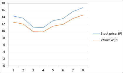
Stock price: (P) | Value: V (P) |
|---|---|
14.3 | 12.52 |
13.69 | 12.01 |
11.08 | 9.82 |
10.98 | 9.74 |
12.97 | 11.41 |
13.6 | 11.94 |
15.6 | 13.6 |
16.71 | 14.56 |
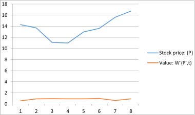
Stock price: () | Value: |
|---|---|
14.3 | 0.55 |
13.69 | 0.917 |
11.08 | 0.939 |
10.98 | 0.902 |
12.97 | 0.931 |
13.6 | 0.976 |
15.6 | 0.64 |
16.71 | 0.9 |
ARCH | AutoRegressive Conditionally Heteroscedastic |
MF-DCCA | Multi-Fractal Detrended Cross-Correlation Analysis |
MMAR | Multi-Fractal Model of Assets Returns |
MSM | Multi-fractal Spectrum Model |
SDE | Stochastic Differential Equation |
| [1] | Mandelbrot, B. B., (1982). The fractal geometry of nature. New York: Freeman. |
| [2] | Jia, L., Xu, W., Linliu, Z., & Qianying, F. (2021). Research on the Portfolio Model based on Mean-MF-DCCA under Multifractal Fea-ture Constraint. Journal of Computational and Applied Mathematics, 386, 113264. |
| [3] | Calvet, L., Fisher, A., & Mandelbrot, B. B. (1997). A multifractal model of asset returns. Working Paper: Yale University. |
| [4] | Mandelbrot, B. B., (1997). Fractals and scaling in finance: Discon-tinuity, Concentration, Risk New York: Springer-Verlag. |
| [5] | Mandelbrot, B. B., Fisher, A., & Calvet, L., (1997). A multifractal model of asset returns. Discussion Paper, Cowles Foundation Yale University. 1164-1166. |
| [6] | Melino, A., (1994). Estimation of continuous-time models in finance, in advances in econometrics: Sixth World Congress. Cambridge. Cambridge University Press. |
| [7] | Drost, F. C., & Werker, B. J. (1996). Closing the GARCH gap: Con-tinuos time GARCH modeling. Journal of Econometrics, 74, 59-84. |
| [8] | Rossi, P. E., (1997). Modeling stock market volatility: Bridging the gap to continuous time. New York: Academic Press. |
| [9] | Wiggins, J. B., (1987). Option values under stochastic volatility: Theory and empirical estimates. Journal of Financial Economics, 19 (2), 351-372. |
| [10] | Taylor, S. J., & Steven, (2008). Modeling financial time series (2nd ed.). New Jersey: World Scientist. |
| [11] | Hamilton, J. D., (2008). Regime-Switching models: New Palgrave Dictionary of Economics (2nd ed.). Palgrave: McMillan Ltd. |
| [12] | Mandelbrot, B. B., (1983). The fractal geometry of nature (Updated and augm. ed.). New York: Freeman. |
| [13] | Mandelbrot, B. B., (2006). Intermittent turbulence in self-similar cascades: Divergence of high moments and dimension of the carrier. Journal of Fluid Mechanics, 62 (2), 331-358. |
| [14] | Mandelbrot, B. B., & Berger, J. M., (1999). Multifractals and 1/f noise: wild self-affinity in physics (1963-1976). (Repr. ed.). New York, NY [u. a.]: Springer. |
| [15] | Eberlein, E., & Keller, U. (1995). Hyperbolic distributions in finance. Bernoulli, 1(3), 281-299. |
| [16] | Calvet, L. E., & Fisher, A. J. (2004). How to forecast long-run vola-tility: Regime switching and the estimation of multifractal processes. Journal of Financial Econometrics, 2, 49-83. |
| [17] | Calvet, L. E., & Fisher, A. J. (1996). Multifractality in assets returns: Theory and evidence. Working paper: Yale University. |
| [18] | Osu, B. O. & Adindu-Dick J. I. (2014). Optimal prediction of the expected value of assets under fractal scaling exponent. Applied Mathematics and Sciences: An International Journal (MathSJ.), Vol. 1, No 3, 41-51. |
APA Style
Adindu-Dick, J. I. (2025). Derivation of Worth Growth Rate of an Investor’s Portfolio Under Multi-fractal Analysis. American Journal of Applied Mathematics, 13(6), 428-437. https://doi.org/10.11648/j.ajam.20251306.15
ACS Style
Adindu-Dick, J. I. Derivation of Worth Growth Rate of an Investor’s Portfolio Under Multi-fractal Analysis. Am. J. Appl. Math. 2025, 13(6), 428-437. doi: 10.11648/j.ajam.20251306.15
AMA Style
Adindu-Dick JI. Derivation of Worth Growth Rate of an Investor’s Portfolio Under Multi-fractal Analysis. Am J Appl Math. 2025;13(6):428-437. doi: 10.11648/j.ajam.20251306.15
@article{10.11648/j.ajam.20251306.15,
  author = {Joy Ijeoma Adindu-Dick},
  title = {Derivation of Worth Growth Rate of an Investor’s Portfolio Under Multi-fractal Analysis},
  journal = {American Journal of Applied Mathematics},
  volume = {13},
  number = {6},
  pages = {428-437},
  doi = {10.11648/j.ajam.20251306.15},
  url = {https://doi.org/10.11648/j.ajam.20251306.15},
  eprint = {https://article.sciencepublishinggroup.com/pdf/10.11648.j.ajam.20251306.15},
  abstract = {The fractal dimension is the basic notion for describing structures that have a scaling symmetry. In finance, multi-fractality is one of the well known facts which characterized non-trivial properties of financial time series. The stock price (or index) fluctuations can be described in terms of long-range temporal correlations by a spectrum of the Holder exponents and a set of fractal dimensions. To forecast the market risk, assessing the stock price indices is the foundation. Multi-fractal has lots of advantages when explaining the volatility of the stock prices. The asset price returns are multi-period market depending on market scenarios which are the measure points. In this work, we use some tools of multi-fractal analysis to derive the worth growth rate of an investor’s portfolio for particular and general cases. For the particular case, we considered the situation when the mean interest rate of some stocks does not depend on other stocks in the market. That is, an investor has invested his money in a stock with a linear mean return. Under the general case, we considered a market comprising some units of assets in long position and a unit of the option in short position. Using Ito’s formula on the present value of the market, we derived the growth rate of investor’s portfolio. Our model equations, which are based on multiplicative processes, capture all the features of the returns. They are tested using data from Zenith Bank of Nigeria stock prices. From our graphs, the worth of investment grows as stock price increases and also decreases with stock price.},
 year = {2025}
}
TY  - JOUR
T1  - Derivation of Worth Growth Rate of an Investor’s Portfolio Under Multi-fractal Analysis
AU  - Joy Ijeoma Adindu-Dick
Y1  - 2025/12/17
PY  - 2025
N1  - https://doi.org/10.11648/j.ajam.20251306.15
DO  - 10.11648/j.ajam.20251306.15
T2  - American Journal of Applied Mathematics
JF  - American Journal of Applied Mathematics
JO  - American Journal of Applied Mathematics
SP  - 428
EP  - 437
PB  - Science Publishing Group
SN  - 2330-006X
UR  - https://doi.org/10.11648/j.ajam.20251306.15
AB  - The fractal dimension is the basic notion for describing structures that have a scaling symmetry. In finance, multi-fractality is one of the well known facts which characterized non-trivial properties of financial time series. The stock price (or index) fluctuations can be described in terms of long-range temporal correlations by a spectrum of the Holder exponents and a set of fractal dimensions. To forecast the market risk, assessing the stock price indices is the foundation. Multi-fractal has lots of advantages when explaining the volatility of the stock prices. The asset price returns are multi-period market depending on market scenarios which are the measure points. In this work, we use some tools of multi-fractal analysis to derive the worth growth rate of an investor’s portfolio for particular and general cases. For the particular case, we considered the situation when the mean interest rate of some stocks does not depend on other stocks in the market. That is, an investor has invested his money in a stock with a linear mean return. Under the general case, we considered a market comprising some units of assets in long position and a unit of the option in short position. Using Ito’s formula on the present value of the market, we derived the growth rate of investor’s portfolio. Our model equations, which are based on multiplicative processes, capture all the features of the returns. They are tested using data from Zenith Bank of Nigeria stock prices. From our graphs, the worth of investment grows as stock price increases and also decreases with stock price.
VL  - 13
IS  - 6
ER  -
Department of Mathematics, Imo State University, Owerri, Nigeria